
This post has been updated on April, 24 2019.
(Brief) Introduction
In this three-series post, I’ll refer to a family of clustering methods that combine dimension reduction with clustering of the observations in data sets with continuous, categorical or mixed-type variables. These methods are implemented in R with our CRAN package clustrd version >1.3 (Markos, Iodice D’Enza and van de Velden, 2018). For data sets with continuous variables, the package provides implementations of Factorial K-means (Vichi and Kiers 2001) and Reduced K-means (De Soete and Carroll 1994); both methods combine Principal Component Analysis (PCA) with K-means clustering. For data sets with categorical variables, MCA K-means (Hwang, Dillon and Takane 2006), iFCB (Iodice D’Enza and Palumbo 2013) and Cluster Correspondence Analysis (van de Velden, Iodice D’Enza and Palumbo 2017) are available; these methods combine variants of (Multiple) Correspondence Analysis (MCA) with K-means. For data sets with both continuous and categorical variables, it provides mixed Reduced K-means and mixed Factorial K-means (van de Velden, Iodice D’Enza and Markos 2019), which combine PCA for mixed-type data with K-means.
Note that the combination of dimension reduction methods (e.g., PCA/MCA) with distance-based clustering techniques (e.g., hierarchical clustering, K-means) is a common strategy and is usually performed in two separate steps: PCA/MCA is applied first to the data at hand and a clustering algorithm is subsequently applied to the factor scores obtained from the first step. This approach, however, known as tandem analysis, may not be always optimal, as the dimension reduction step optimises a different objective function from the clustering step. As a result, dimension reduction may mask the clustering structure. The ineffectiveness of tandem analysis has been argued by Arabie and Hubert (1994), Milligan (1996), Dolnicar and Grün (2008) and van de Velden et al. (2017), among others. On the contrary, joint dimension reduction and clustering techniques combine the two criteria (dimension reduction and clustering) into a single objective function, which can be optimized via Alternating Least Squares (ALS). For more details see, e.g. van de Velden et al. (2017), Markos et al. (2018), and van de Velden et al. (2019).
The clustrd package contains three main functions: cluspca(), clusmca() and cluspcamix() for data sets with continuous, categorical and mixed-type variables, respectively. The package also contains three functions for cluster validation, tuneclus(), global_bootclus() and local_bootclus().
In this post, I will demonstrate cluspca(), a function that implements joint dimension reduction and clustering for continuous data, as well as the three functions for cluster validation.
Reduced K-means on the Iris data set
Let’s try to cluster a set of observations described by continuous variables. How about the Iris flower data set? If you are now screaming “not this one again!”, please be patient - that’s a convenient choice to demonstrate a clustering method.
We begin with installing and loading the package:
# installing clustrd
install.packages("clustrd")
# loading clustrd
library(clustrd)
The cluspca() function has three arguments that must be provided: a data.frame (data), the number of clusters (nclus) and the number of dimensions (ndim). Optional arguments include alpha, method, center, scale, rotation, nstart, smartStart and seed, described below.
alpha is a scalar between 0 and 1; alpha = 0.5 leads to Reduced K-means, alpha = 0 to Factorial K-means, and alpha = 1 reduces to the tandem approach (PCA followed by K-means). alpha can also take intermediate values between 0 and 1, adjusting for the relative importance of RKM and FKM in the objective function. The default value of alpha is 0.5 (Reduced K-means).
method can be either “RKM” for Reduced K-means or “FKM” for Factorial K-means (default is “RKM”)
center and scale are logicals indicating whether the variables should be shifted to be zero centered or have unit variance, respectively.
rotation specifies the method used to rotate the factors. Options are “none” for no rotation, “varimax” for varimax rotation with Kaiser normalization and “promax” for promax rotation (default = “none”)
nstart indicates the number of iterations (default is 100)
smartStart can accept a cluster membership vector as a starting solution (default is NULL, where a starting solution is randomly generated) - note that these methods are iterative and a smart initialization can help.
seed is an integer used as argument by set.seed() for offsetting the random number generator when smartStart = NULL. The default value is 1234.
We set the number of clusters to 3 and the number of dimensions to 2 (in fact, setting the number of dimensions to the number of clusters minus 1 is recommended in the literature).
# apply Reduced K-means to iris (class variable is excluded)
out.cluspca = cluspca(iris[,-5], 3, 2, seed = 1234)
summary(out.cluspca)
Here’s a summary of the solution:
Solution with 3 clusters of sizes 53 (35.3%), 50 (33.3%), 47 (31.3%) in 2 dimensions.
Variables were mean centered and standardized.

Cluster centroids:
            Dim.1   Dim.2
Cluster 1  0.5896  0.7930
Cluster 2 -2.2237 -0.2380
Cluster 3  1.7008 -0.6411

Variable scores:
               Dim.1   Dim.2
Sepal.Length  0.5014 -0.4359
Sepal.Width  -0.2864 -0.8973
Petal.Length  0.5846  0.0024
Petal.Width   0.5699 -0.0699

Within cluster sum of squares by cluster:
[1] 34.5002 44.3823 34.4589
 (between_SS / total_SS =  80.13 %)

Clustering vector:
  [1] 2 2 2 2 2 2 2 2 2 2 2 2 2 2 2 2 2 2 2 2 2 2 2 2 2 2 2 2 2 2 2
 [32] 2 2 2 2 2 2 2 2 2 2 2 2 2 2 2 2 2 2 2 3 3 3 1 1 1 3 1 1 1 1 1
 [63] 1 1 1 3 1 1 1 1 3 1 1 1 1 3 3 3 1 1 1 1 1 1 1 3 3 1 1 1 1 1 1
 [94] 1 1 1 1 1 1 1 3 1 3 3 3 3 1 3 3 3 3 3 3 1 1 3 3 3 3 1 3 1 3 1
[125] 3 3 1 3 3 3 3 3 3 1 1 3 3 3 1 3 3 3 1 3 3 3 1 3 3 1

Objective criterion value: 69.4442

Available output:

 [1] "obscoord"  "attcoord"  "centroid"  "cluster"   "criterion" "size"      "odata"     "scale"
 [9] "center"    "nstart"
An important feature of Reduced K-means is that we can visualize observations, cluster centers and variables on a low-dimensional space, similar to PCA.
# plotting the RKM solution
plot(out.cluspca, cludesc = TRUE)
This creates a biplot of observations and variables as shown below. Note that cludesc = TRUE creates a parallel coordinate plot to facilitate cluster interpretation. For help(plot.cluspca)
Reduced K-means biplot of observations (points) and variables (biplot axes) of the Iris data set with respect to components 1 (horizontal) and 2 (vertical). Cluster means are labelled C1 through C3.
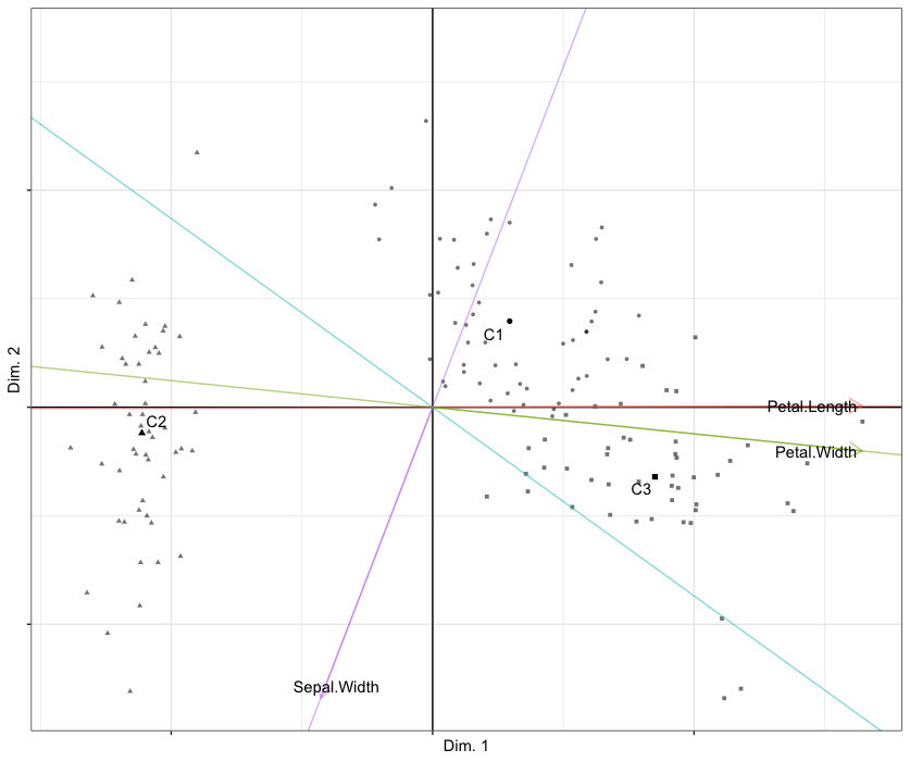
It is helpful to compute the confusion matrix between the true cluster partition (iris[, 5]) and the one obtained by Reduced K-means (out.cluspca$cluster). The agreement between the obtained partition and the true partition is moderate, according to an adjusted Rand index of .62.
table(iris[, 5],out.cluspca$cluster)
1 2 3
setosa 0 50 0
versicolor 39 0 11
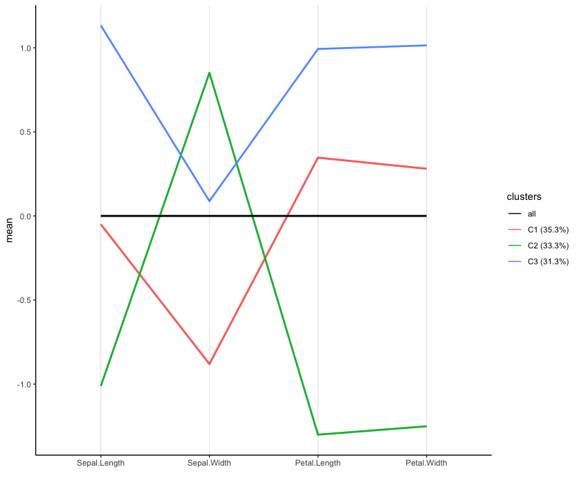
virginica 14 0 36The parallel coordinate plot (shown below) depicts cluster means for each variable and provides quick insights into the differences between groups. The mean values, depicted on the vertical axis, correspond to mean centered and standardized variables. All instances of setosa are in the second cluster having large sepal width and low petal length and width, compared to the other clusters. The first cluster contains most instances of versicolor (39 out of 50), characterized by low sepal width. Most instances of virginica (36 out of 50) are in the third cluster, having high sepal length, petal length and petal width.
Parallel coordinate plot of the cluster means (line thickness is proportional to cluster size).
Choosing the number of clusters and dimensions
In the case of Iris data, where the true clusters are known, the decision on the number of clusters and dimensions is more or less obvious. In many cases, however, the selection of the most appropriate number of clusters and dimensions requires a careful assessment of solutions corresponding to different parameter choices. To facilitate a quantitative appraisal of solutions corresponding to different parameter settings, the clustrd package provides the function tuneclus(). The function requires a dataset (data argument), the range of clusters (nclusrange) and dimensions (ndimrange), as well as the desired method, through the method argument.
The function provides two well-established distance-based statistics to assess the quality of an obtained clustering solution via the criterion argument; the overall average silhouette width (ASW) index (criterion = “asw”) and the Calinski-Harabasz (CH) index (criterion = “ch”). The ASW index, which ranges from −1 to 1, reflects the compactness of the clusters and indicates whether a cluster structure is well separated or not. The CH index is the ratio of between-cluster variance to within-cluster variance, corrected according to the number of clusters, and takes values between 0 and infinity. In general, the higher the ASW and CH values, the better the cluster separation. Also, the function allows the specification of the data matrix used to compute the distances between observations, via the dst argument. When dst = “full” (default) the appropriate distance measure is computed on the original data. In particular, the Euclidean distance is used for continuous variables and Gower’s distance for categorical variables. When the option is set to “low”, the distance is computed between the low-dimensional object scores.
To demonstrate parameter tuning, we apply Reduced K-means to the Iris data for a range of clusters between 3 and 5 and dimensions ranging from 2 to 4. The Euclidean distance was computed between observations on the low dimensional space (dst = “low”). The average silhouette width was used as a cluster quality assessment criterion (criterion = “asw”). As shown below, the best solution was obtained for 3 clusters and 2 dimensions.
# Cluster quality assessment based on the average silhouette width
# in the low dimensional space
bestRKM = tuneclus(iris[,-5], 3:5, 2:4, method = "RKM", criterion = "asw",
          dst = "low")
bestRKM
The best solution was obtained for 3 clusters of sizes 53 (35.3%), 50 (33.3%),
47 (31.3%) in 2 dimensions, for a cluster quality criterion value of 0.511.
Variables were mean centered and standardized.
Cluster quality criterion values across the specified range of clusters (rows)
and dimensions (columns):
2 3 4
3 0.511
4 0.444 0.424
5 0.413 0.359 0.342
Cluster centroids:
Dim.1 Dim.2
Cluster 1 0.5896 0.7930
Cluster 2 -2.2237 -0.2380
Cluster 3 1.7008 -0.6411
Within cluster sum of squares by cluster:
[1] 34.5002 44.3823 34.4589
(between_SS / total_SS = 80.13 %)
Objective criterion value: 69.4442
Available output:
[1] "clusobjbest" "nclusbest" "ndimbest" "critbest" "critgrid"The “best” solution can be subsequently plotted.
plot(bestRKM)Assessing Cluster Stability
Cluster stability is an important aspect of cluster validation. Our focus is on stability assessment of a partition, that is, given a new sample from the same population, how likely is it to obtain a similar clustering? Stability can also be used to select the number of clusters because if true clusters exist, the corresponding partition should have a high stability. Resampling approaches (that is, bootstrapping, subsetting, replacement of points by noise) provide an elegant framework to computationally derive the distribution of interesting quantities describing the quality of a partition (Hennig, 2007; Dolnicar and Leisch, 2017).
The functions global_bootclus() and local_bootclus() can be used for assessing global and local cluster stability, respectively, via bootstrapping. “Global” here refers to the stability of each partition over a range of clustering number choices, e.g., from 2 to 5 clusters. “Local” stability, instead, refers to the stability of each one of the clusters in a single partition.
The algorithm implemented in global_bootclus() is similar to that of Dolnicar and Leisch (2010) and can be summarized as follows: two bootstrap samples of size n, the number of observations, are drawn with replacement from the original data set. Then, for a prespecified number of clusters and a number of dimensions, a joint dimension reduction and clustering method is applied to each sample and two clustering partitions are obtained. Subsequently, each one of the original observations is assigned to the closest center of each one of the obtained clustering partitions, using the Euclidean distance, and two new partitions are obtained. Stability is defined as the degree of agreement between these two final partitions and can be evaluated via the Adjusted Rand Index (ARI; Hubert & Arabie, 1985) or the Measure of Concordance (MOC; Pfitzner, Leibbrandt, & Powers, 2009) as measure of agreement and stability. This procedure is repeated many times (e.g., 100) and the distributions of ARI and MOC can be inspected to assess the global reproducibility of different solutions.
Let’s go back to the Iris data and assess global stability of reduced K-means from 2 to 4 clusters. The number of bootstrap pairs of partitions (nboot) is set to 20 and the number of starts of RKM to 50. While nboot = 100 is recommended, smaller run numbers could give quite informative results as well, if computation times become too high. Notice that ndim, the dimensionality of the solution, is missing; in this case, it is set internally to nclus - 1, but it can also be user-defined.
# Global stability assessment: Reduced K-means from 2 to 4 clusters
data(iris)
boot_RKM = global_bootclus(iris[,-5], nclusrange = 2:4,
method = "RKM", nboot = 20, nstart = 50, seed = 1234)
summary(boot_RKM$rand)
This code will take some time to execute, since it will evaluate the two-, three- and four-cluster solutions for 20 bootstrap replicates.
2 3 4
Min. :0.9466 Min. :0.5822 Min. :0.4504
1st Qu.:0.9731 1st Qu.:0.7158 1st Qu.:0.5204
Median :0.9731 Median :0.8117 Median :0.6425
Mean :0.9799 Mean :0.7961 Mean :0.6496
3rd Qu.:1.0000 3rd Qu.:0.8731 3rd Qu.:0.7644
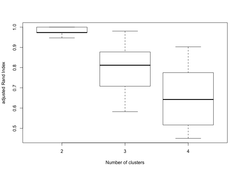
Max. :1.0000 Max. :0.9803 Max. :0.9026A summary of the ARI distributions for 2, 3 and 4 clusters reveals that the two-cluster solution is the most stable, followed by the three-cluster and the four-cluster solutions. A visual inspection of the corresponding boxplots also confirms this finding. This result is not surprising since the Iris data set only contains two clusters with rather obvious separation. One of the clusters contains Iris setosa, while the other cluster contains both Iris virginica and Iris versicolor and is not separable without the species information Fisher used.
boxplot(boot_RKM$rand, xlab = "Number of clusters", ylab = "adjusted Rand Index")Global stability of Reduced K-means solutions (K = 2 to 4).
The algorithm implemented in local_bootclus() is similar to that of Hennig (2007) and can be summarized as follows: For a prespecified number of clusters and a number of dimensions, a joint dimension reduction and clustering method is applied to the original data. Then, two bootstrap samples of size n, the number of observations, are drawn with replacement from the original data set. The method is applied to each sample and two clustering partitions are obtained. Subsequently, each one of the original observations is assigned to the closest center of each one of the obtained clustering partitions, using the Euclidean distance, and two new partitions are obtained. The maximum Jaccard agreement between each original cluster and each one of the two partitions is calculated. The average of each pair is taken as a measure of “local” or cluster-wise stability. This procedure is repeated many times (e.g., 100) and the distributions of the Jaccard similarity can be inspected to assess the stability of each cluster in the solution.
Here are some guidelines for interpretation. Generally, a valid, stable cluster should yield a mean Jaccard similarity value of 0.75 or more. Between 0.6 and 0.75, clusters may be considered as indicating patterns in the data, but which points exactly should belong to these clusters is highly doubtful. Below average Jaccard values of 0.6, clusters should not be trusted. “Highly stable” clusters should yield average Jaccard similarities of 0.85 and above.
For the Iris data, we will now assess the local stability of the three-clusters obtained via Reduced K-means (nclus = 3, ndim = 2).
# Cluster-wise stability assessment: Reduced K-means from 2 to 4 clusters
data(iris)
bootres = local_bootclus(iris[,-5], nclus = 3, ndim = 2,
method = "RKM", nboot = 20, nstart = 50, seed = 1234)
summary(bootres$Jaccard)
1 2 3
Min. :0.6238 Min. :1 Min. :0.6908
1st Qu.:0.7352 1st Qu.:1 1st Qu.:0.7441
Median :0.7770 Median :1 Median :0.7641
Mean :0.7682 Mean :1 Mean :0.7616
3rd Qu.:0.8083 3rd Qu.:1 3rd Qu.:0.7830
Max. :0.8468 Max. :1 Max. :0.8036Obviously, all clusters are stable and the second cluster is the most stable with an average stability of 1 (the maximum possible). This cluster contains the 50 observations of Iris setosa. The other two clusters are also quite stable.
boxplot(bootres$Jaccard, xlab = "cluster number", ylab = "Jaccard similarity (cluster stability)")Local stability of a Reduced K-means solution with 3 clusters in 2 dimensions.

Epilogue
For a thorough treatment of joint dimension reduction and clustering methods and additional applications you can read our JSS and WIREs papers. Note, however, that cluster stability is not discussed in any of these papers, since this functionality was added to the package later on. The clustrd package is still evolving; ongoing refinements, new features and fixing bugs are being enhanced regularly. Any feedback will be much appreciated.
In follow-up posts, I demonstrate the application of joint dimension reduction and clustering to categorical and mixed-type data sets.
References
Arabie, P., & Hubert, L. (1994). Cluster Analysis in Marketing Research. In R. P. Bagozzi. (Ed.), Advanced Methods of Marketing Research (pp. 160-189). Cambridge: Blackwell.
De Soete, G., & Carroll, J. D. (1994). K-means clustering in a low-dimensional euclidean space. In E. Diday, Y. Lechevallier, M. Schader, P. Bertrand, & B. Burtschy (Eds.), New Approaches in Classification and Data Analysis (pp. 212-219). Springer-Verlag, Berlin.
Dolnicar, S., & Grün, B. (2008). Challenging “factor–cluster segmentation”. Journal of Travel Research, 47(1), 63-71.
Dolnicar, S., & Leisch, F. (2010). Evaluation of structure and reproducibility of cluster solutions using the bootstrap. Marketing Letters, 21(1), 83-101.
Dolnicar, S., & Leisch, F. (2017). Using segment level stability to select target segments in data-driven market segmentation studies. Marketing Letters, 28(3), 423-436.
Hennig, C. (2007). Cluster-wise assessment of cluster stability. Computational Statistics and Data Analysis, 52, 258-271.
Hwang, H., Dillon, W. R., & Takane, Y. (2006). An Extension of Multiple Correspondence Analysis for Identifying Heterogenous Subgroups of Respondents. Psychometrika, 71, 161-171.
Iodice D’Enza, A., & Palumbo, F. (2013). Iterative factor clustering of binary data. Computational Statistics, 28(2), 789-807.
Markos, A., Iodice D’Enza, A., & van de Velden, M. (2018). Beyond Tandem Analysis: Joint Dimension Reduction and Clustering in R. Journal of Statistical Software (accepted for publication).
Milligan, G. W. (1996). Clustering validation: results and implications for applied analyses. In P. Arabie, L. J. Hubert (Eds.), Clustering and classification (pp. 341-375). River Edge: World Scientific Publications.
Pfitzner, D., Leibbrandt, R., & Powers, D. (2009). Characterization and evaluation of similarity measures for pairs of clusterings. Knowledge and Information Systems, 19(3), 361-394.
van de Velden, M., Iodice D’Enza, A., & Palumbo, F. (2017). Cluster Correspondence Analysis. Psychometrika, 82(1), 158-185.
van de Velden, M., Iodice D’Enza, A., & Markos, A. (2019). Distance-based clustering of mixed data. WIREs Computational Statistics, 11(3), e1456. DOI:10.1002/wics.1456.
Vichi, M., Vicari, D., & Kiers, H.A.L. (2019). Clustering and dimension reduction for mixed variables. Behaviormetrika doi:10.1007/s41237-018-0068-6.
Vichi, M., & H. A. (2001). Factorial k-means analysis for two-way data. Computational Statistics & Data Analysis, 37(1), 49-64.